nall <- nrow(race) + nrow(skin) + nrow(age) + nrow(weight) +
    nrow(sexuality) + nrow(usa) + nrow(gender_science) + nrow(ethnic)
The Israeli site on Project Implicit has included eight IATs about the following topics (the N refers to the number of sessions I analyzed):
- Race: ‘Black - White’ IAT (N = 3902)
- Ethnicity: ‘Ashkenazi - Mizrahi’ IAT (N = 8037)
- Skin-tone: ‘Light Skin - Dark Skin’ IAT (N = 3175)
- Age: ‘Young - Old’ IAT (N = 2903)
- Sexuality: ‘Gay - Straight’ IAT (N = 5792)
- Weight: ‘Fat - Thin’ IAT (N = 5155)
- Nationalism: ‘USA - Own Country’ IAT (N = 2143)
- Gender - Science: ‘Male+Science - Female+Liberal arts’ IAT (N = 5022)
The attributes used on all IATs except Gender - Science are Good vs. Bad.
A common interpretation of the IAT score for each of these tasks is that it reflects the strength of association between the categories and the attributes used in the task (for example, an association between Young people + Good and Old people + Bad).
Some researchers interpret this strength of association as the participants’ implicit or automatic preference between the two categories/ an automatic bias in judgment (but see disclaimer below). In this post, I will be conservative in my interpretation, and thus refer to IAT scores in a certain direction (rather than zero) as reflecting bias in IAT scores.
Each task also included 1 or 2 self-reported judgment measures:
- Self-Reported Direct Preference: Preference between the dominant and non-dominant category (scale: 1 = “I strongly prefer NON-DOMINANT CATEGORY to DOMINANT CATEGORY to 7 =”I strongly prefer DOMINANT CATEGORY to NON-DOMINANT CATEGORY")
- Feeling Thermometer: Cold to warm feelings toward each category (scale: 0 “very cold” to 10 “very warm”). We computed a difference score of dominant category - non-dominant category.
The tasks also included secondary measures such as perception measures and demographic items. You can check out the data and codebooks on OSF!
I analyzed the results of each task, from 12 years of data collection (2009-2020) and a total of 36129 participants. I found a robust and persistent pro-dominant bias: The IAT scores from all tasks revealed that Israelis strongly associate the dominant social groups (e.g., White people, Ashkenazi people, Young people) with positive attributes and the non-dominant social groups (Black people, Mizrahi people, Old people) with negative attributes. The results from my analyses could be used as a first step in the examination of (supposedly) automatic biases against groups in Israel and of the most prominent bias in this country (that is, the task with the largest difference between the two groups/categories). This would be a first step as Project Implicit’s samples are not representative samples, and because it would be preferable to test the generalizability of automatic bias beyond the IAT scores.
IAT Scores per Task
All tasks point to a pro-dominant association. Israelis showed the strongest bias in their IAT scores in the Nationalism IAT (Own Country > USA), followed by Age (Young > Old), and the Gender-Science stereotypes (Male+Science - Female+Liberal arts > Male+Liberal arts - Female+Science). The smallest bias was in the Sexuality IAT (Straight > Gay people) and Weight IAT (Thin > Fat):
Note. The plot below shows the effect-size (Cohen’s d; not the IAT D score) as a function of the IAT task. Larger effect-sizes indicate a stronger pro-dominant bias. The effect-size is based on IAT scores computed with the D2 scoring algorithm. The data also contains the D6 score (the scores are strongly correlated, r = 0.96-0.98).
race$IAT <- race$D2.D.White_Good_all
skin$IAT <- skin$D2.D.LightSkin_Good_all
age$IAT <- age$D2.D.Young_Good_all
sexuality$IAT <- sexuality$D2.D.Straight_Good_all
weight$IAT <- weight$D2.D.Thin_Good_all
usa$IAT <- usa$D2.D.Own_Good_all
gender_science$IAT <- gender_science$D2.D.Male_Science_all
ethnic$IAT <- ethnic$D2.D.Ash_Good_all
aget <- ttestOneS(age, vars = vars(IAT), testValue = 0, effectSize = T)
aget <- as.data.frame(aget$ttest)
aged <- round(aget[[6]], 2)
racet <- ttestOneS(race, vars = vars(IAT), testValue = 0, effectSize = T)
racet <- as.data.frame(racet$ttest)
raced <- round(racet[[6]], 2)
skint <- ttestOneS(skin, vars = vars(IAT), testValue = 0, effectSize = T)
skint <- as.data.frame(skint$ttest)
skind <- round(skint[[6]], 2)
weightt <- ttestOneS(weight, vars = vars(IAT), testValue = 0,
effectSize = T)
weightt <- as.data.frame(weightt$ttest)
weightd <- round(weightt[[6]], 2)
ethnict <- ttestOneS(ethnic, vars = vars(IAT), testValue = 0,
effectSize = T)
ethnict <- as.data.frame(ethnict$ttest)
ethnicd <- round(ethnict[[6]], 2)
sexualityt <- ttestOneS(sexuality, vars = vars(IAT), testValue = 0,
effectSize = T)
sexualityt <- as.data.frame(sexualityt$ttest)
sexualityd <- round(sexualityt[[6]], 2)
usat <- ttestOneS(usa, vars = vars(IAT), testValue = 0, effectSize = T)
usat <- as.data.frame(usat$ttest)
usad <- round(usat[[6]], 2)
gen_sci_t <- ttestOneS(gender_science, vars = vars(IAT), testValue = 0,
effectSize = T)
gen_sci_t <- as.data.frame(gen_sci_t$ttest)
gen_sci_d <- round(gen_sci_t[[6]], 2)
all_ds <- c(aged, raced, skind, weightd, ethnicd, sexualityd,
usad, gen_sci_d) %>% as.data.frame()
colnames(all_ds) <- "es"
all_ds$Task <- c("Age", "Race", "Skin", "Weight", "Ethnicity",
"Sexuality", "Nationalism", "Gender-Science")pp <- ggdotchart(all_ds, x = "Task", y = "es",
color = "Task", # Color by groups
ylab = "Cohen's d",
#palette = c("#00AFBB", "#E7B800", "#FC4E07"), # Custom color palette
sorting = "descending", # Sort value in descending order
add = "segments", # Add segments from y = 0 to dots
rotate = TRUE, # Rotate vertically
#group = "cyl", # Order by groups
dot.size = 30, # Large dot size
label = round(all_ds$es,3), # Add mpg values as dot labels
font.label = list(color = "white", size = 25,
vjust = 0.5), # Adjust label parameters
ggtheme = theme_pubr() # ggplot2 theme
)
pp <- pp + geom_hline(yintercept = 0, linetype = "dashed", color = "darkblue",
size = 1.2)
pp <- pp + font("title", size = 30, color = "black", face = "bold")+
font("legend.text", size = 26, color = "black", face = "bold")+
font("xlab", size = 28, color = "black", face = "bold")+
font("ylab", size = 28, color = "black", face = "bold")+
font("xy.text", size = 25, color = "black", face = "bold")
pp <- pp +theme(legend.position="none")
pp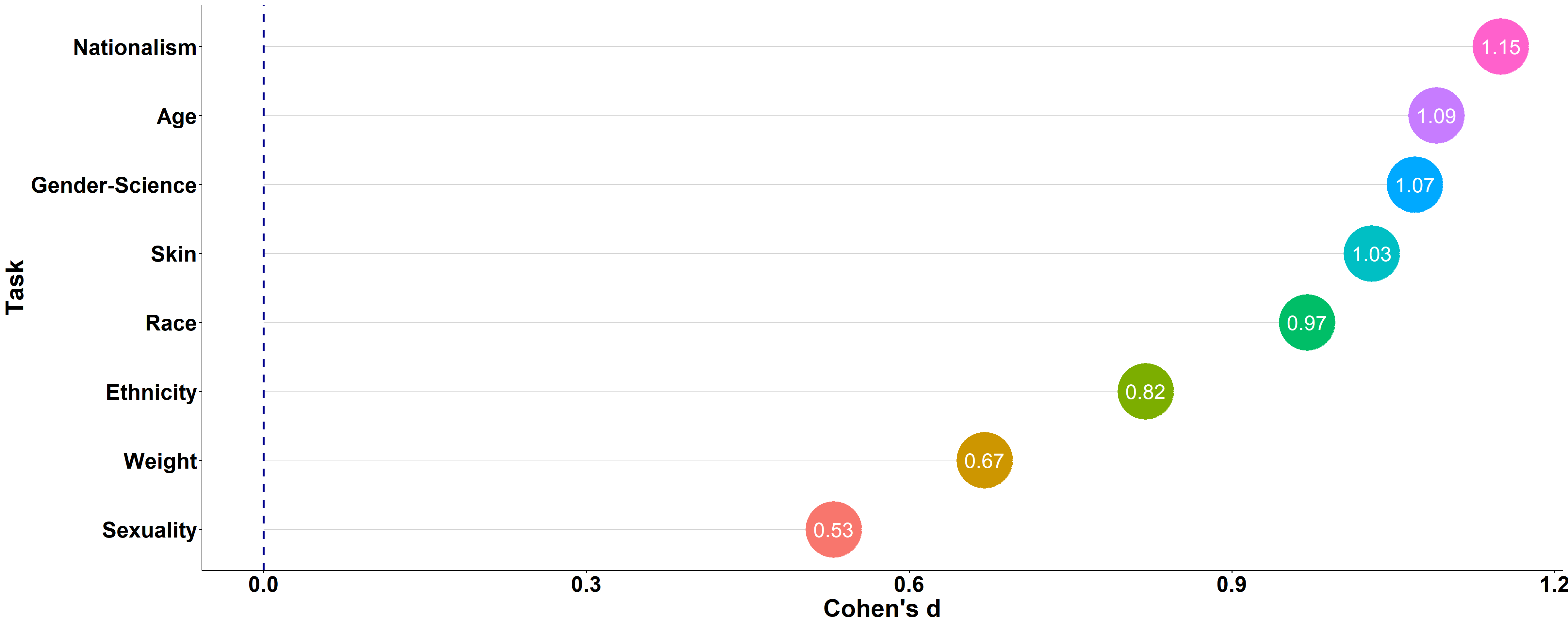
Future studies could explore whether the extent of bias as measured with the IAT relates to the extent of real-world discrimination and to other negative treatment of disadvantaged groups in Israel. A surprising result from this analysis is that the bias regarding Gay people (Sexuality IAT) was relatively small (d = 0.54). This is surprising because Israel is a relatively orthodox country, so a weak anti-Gay bias is less expected. However, remember that Project Implicit’s sample is not representative of the Israeli population. The data I uploaded to the OSF contains demographic variables such as gender-identity, religiosity and ethnicity, that could provide a first clue to the level of anti-Gay bias among different sectors in Israel.
Self-Report Scores per Task
Israelis were often biased in their self-reports, and not just in their IAT scores… but, as might be expected, this bias was a bit weaker in its magnitude. Interestingly, there were some differences between the strongest bias in the IAT scores and in the self-report scores. The strongest self-reported bias among Israeli participants is in the Nationalism (Own Country > USA) study and Weight (Thin > Fat) study, and the smallest bias is in the Sexuality (Straight > Gay people) study, Ethnicity (Ashkenazi > Mizrahi) study, and Age (Young > Old) study:
Self-Reported Direct Preference
Participants reported their preference between the dominant and non-dominant category (scale: 1 = “I strongly prefer NON-DOMINANT CATEGORY to DOMINANT CATEGORY to 7 =”I strongly prefer DOMINANT CATEGORY to NON-DOMINANT CATEGORY").
Note: The plot below shows the effect-size (Cohen’s d) as a function of the direct self-reported preference task. Larger effect-sizes indicate a stronger pro-dominant bias. Not all tasks included the direct self-reported preference measure.
aget <- ttestOneS(age, vars = vars(att), testValue = 4, effectSize = T)
aget <- as.data.frame(aget$ttest)
aged <- round(aget[[6]], 2)

racet <- ttestOneS(race, vars = vars(att), testValue = 4, effectSize = T)
racet <- as.data.frame(racet$ttest)
raced <- round(racet[[6]], 2)

weightt <- ttestOneS(weight, vars = vars(att), testValue = 4,
    effectSize = T)
weightt <- as.data.frame(weightt$ttest)
weightd <- round(weightt[[6]], 2)

ethnict <- ttestOneS(ethnic, vars = vars(att), testValue = 4,
    effectSize = T)
ethnict <- as.data.frame(ethnict$ttest)
ethnicd <- round(ethnict[[6]], 2)

sexualityt <- ttestOneS(sexuality, vars = vars(att), testValue = 4,
    effectSize = T)
sexualityt <- as.data.frame(sexualityt$ttest)
sexualityd <- round(sexualityt[[6]], 2)

usat <- ttestOneS(usa, vars = vars(att), testValue = 4, effectSize = T)
usat <- as.data.frame(usat$ttest)
usad <- round(usat[[6]], 2)


all_ds <- c(aged, raced, weightd, ethnicd, sexualityd, usad) %>%
    as.data.frame()
colnames(all_ds) <- "es"

all_ds$Task <- c("Age", "Race", "Weight", "Ethnicity", "Sexuality",
    "Nationalism")
pp <- ggdotchart(all_ds, x = "Task", y = "es",
color = "Task", # Color by groups
ylab = "Cohen's d",
#palette = c("#00AFBB", "#E7B800", "#FC4E07"), # Custom color palette
sorting = "descending", # Sort value in descending order
add = "segments", # Add segments from y = 0 to dots
rotate = TRUE, # Rotate vertically
#group = "cyl", # Order by groups
dot.size = 30, # Large dot size
label = round(all_ds$es,3), # Add mpg values as dot labels
font.label = list(color = "white", size = 25,
vjust = 0.5), # Adjust label parameters
ggtheme = theme_pubr() # ggplot2 theme
)
pp <- pp + geom_hline(yintercept = 0, linetype = "dashed", color = "darkblue",
size = 1.2)
pp <- pp + font("title", size = 30, color = "black", face = "bold")+
font("legend.text", size = 26, color = "black", face = "bold")+
font("xlab", size = 28, color = "black", face = "bold")+
font("ylab", size = 28, color = "black", face = "bold")+
font("xy.text", size = 25, color = "black", face = "bold")
pp <- pp +theme(legend.position="none")
pp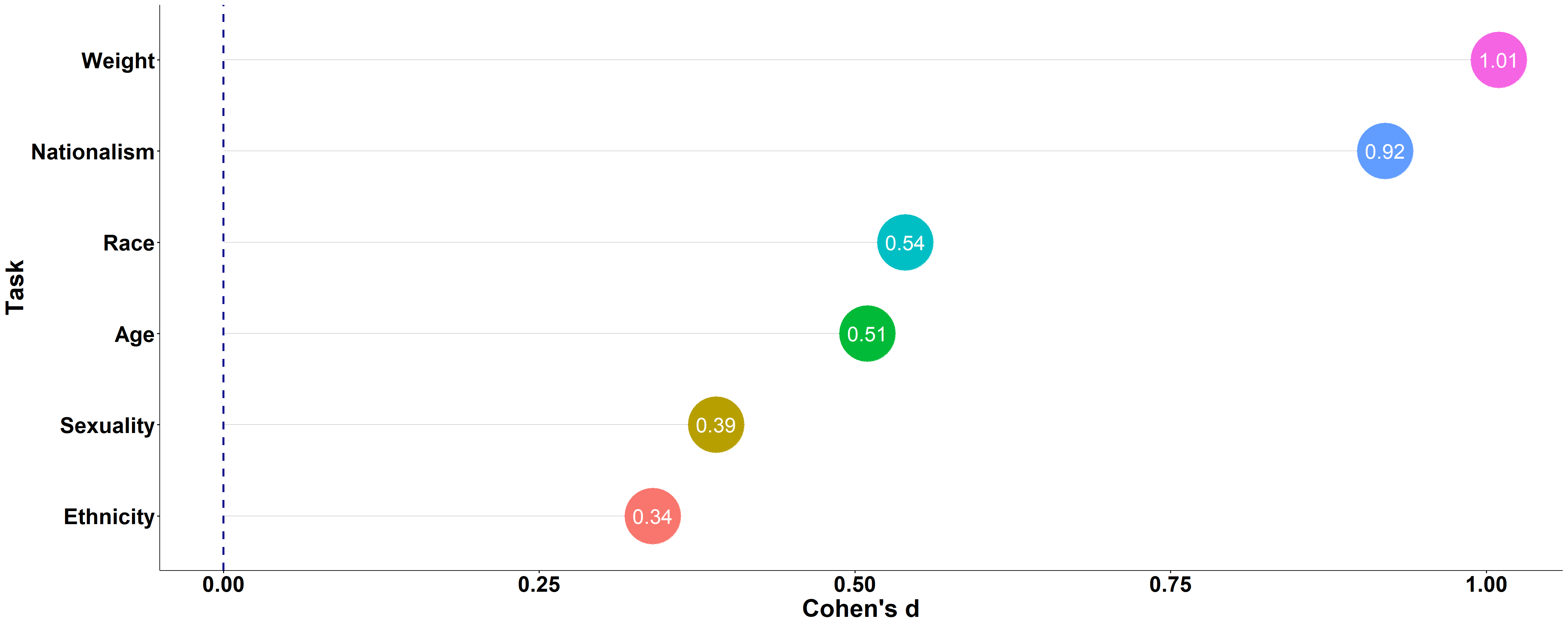
Feeling thermometer (Difference score)
Participants reported their feelings toward each category (scale: 0 “very cold” to 10 “very warm”). We computed a difference score of [dominant category - non-dominant category] as another measure of self-reported preference.
Gender-Science: In this study the scale was 1 = “Strongly female” to 7 = “Strongly male”. The score was computed as the rating for science minus the rating for liberal arts. Higher scores indicate a consideration of science as masculine and liberal arts as feminine.
The effect-sizes on this measure were smaller, compared with the previous measure. This difference might result from the nature of each measure: while the Self-reported preference measure directly compares the two categories (as does the IAT), the thermometer does not compare the two categories directly. A comparative context might facilitate bias.
Note: The plot below shows the effect-size (Cohen’s d) as a function of the feeling thermometer task. Larger effect-sizes indicate a stronger pro-dominant bias. Not all tasks included the feeling thermometer measure.
aget <- ttestOneS(age, vars = vars(diff_thermo), testValue = 0,
    effectSize = T)
aget <- as.data.frame(aget$ttest)
aged <- round(aget[[6]], 2)

racet <- ttestOneS(race, vars = vars(diff_thermo), testValue = 0,
    effectSize = T)
racet <- as.data.frame(racet$ttest)
raced <- round(racet[[6]], 2)

skint <- ttestOneS(skin, vars = vars(diff_thermo), testValue = 0,
    effectSize = T)
skint <- as.data.frame(skint$ttest)
skind <- round(skint[[6]], 2)

weightt <- ttestOneS(weight, vars = vars(diff_thermo), testValue = 0,
    effectSize = T)
weightt <- as.data.frame(weightt$ttest)
weightd <- round(weightt[[6]], 2)

usat <- ttestOneS(usa, vars = vars(diff_thermo), testValue = 0,
    effectSize = T)
usat <- as.data.frame(usat$ttest)
usad <- round(usat[[6]], 2)

gender_sciencet <- ttestOneS(gender_science, vars = vars(diff_thermo),
    testValue = 0, effectSize = T)
gender_sciencet <- as.data.frame(gender_sciencet$ttest)
gender_scienced <- round(gender_sciencet[[6]], 2)

all_ds <- c(aged, raced, skind, weightd, usad, gender_scienced) %>%
    as.data.frame()
colnames(all_ds) <- "es"

all_ds$Task <- c("Age", "Race", "Skin", "Weight", "Nationalism",
    "Gender-Science")
pp <- ggdotchart(all_ds, x = "Task", y = "es",
color = "Task", # Color by groups
ylab = "Cohen's d",
#palette = c("#00AFBB", "#E7B800", "#FC4E07"), # Custom color palette
sorting = "descending", # Sort value in descending order
add = "segments", # Add segments from y = 0 to dots
rotate = TRUE, # Rotate vertically
#group = "cyl", # Order by groups
dot.size = 30, # Large dot size
label = round(all_ds$es,3), # Add mpg values as dot labels
font.label = list(color = "white", size = 25,
vjust = 0.5), # Adjust label parameters
ggtheme = theme_pubr() # ggplot2 theme
)
pp <- pp + geom_hline(yintercept = 0, linetype = "dashed", color = "darkblue",
size = 1.2)
pp <- pp + font("title", size = 30, color = "black", face = "bold")+
font("legend.text", size = 26, color = "black", face = "bold")+
font("xlab", size = 28, color = "black", face = "bold")+
font("ylab", size = 28, color = "black", face = "bold")+
font("xy.text", size = 25, color = "black", face = "bold")
pp <- pp +theme(legend.position="none")
pp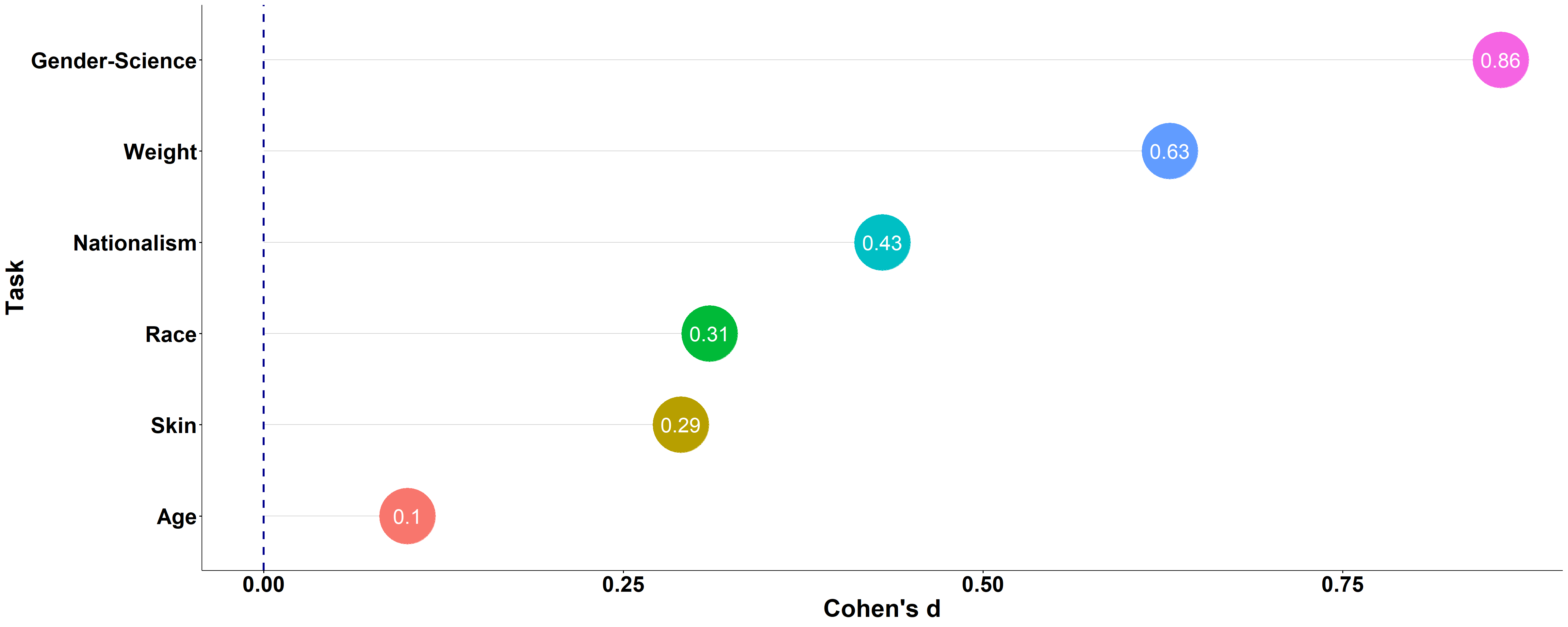
Does that mean that Israelis are more OK with being biased toward Fat people, and in favor of their own country, than toward elderly people, for example? Does that relate to certain social values in the Israeli society? We think these are interesting questions that could be addressed in future research.
Yearly patterns
Do people get better? - Next, I looked at the scores per year, to see if bias decreases throughout the years. I should note that there is no guarantee that the participants came from the same population each year. We do not have much information about the population. We assume that these are mostly students sent by lecturers of intro to social psychology and other courses. Across all years, we can see that self-report and IAT scores favor the dominant groups, and that the bias reflected in the IAT scores is much larger.
age <- age %>% drop_na(year)
age$Year <- as.factor(age$year)

race <- race %>% drop_na(year)
race$Year <- as.factor(race$year)

skin <- skin %>% drop_na(year)
skin$Year <- as.factor(skin$year)

ethnic <- ethnic %>% drop_na(year)
ethnic$Year <- as.factor(ethnic$year)

weight <- weight %>% drop_na(year)
weight$Year <- as.factor(weight$year)

sexuality <- sexuality %>% drop_na(year)
sexuality$Year <- as.factor(sexuality$year)

usa <- usa %>% drop_na(year)
usa$Year <- as.factor(usa$year)

gender_science <- gender_science %>% drop_na(year)
gender_science$Year <- as.factor(gender_science$year)
# verify that sessionId is of the same type across DFs
race$sessionId <- as.character(race$sessionId)
skin$sessionId <- as.character(skin$sessionId)
age$sessionId <- as.character(age$sessionId)
ethnic$sessionId <- as.character(ethnic$sessionId)
sexuality$sessionId <- as.character(sexuality$sessionId)
usa$sessionId <- as.character(usa$sessionId)
gender_science$sessionId <- as.character(gender_science$sessionId)
weight$sessionId <- as.character(weight$sessionId)
race_iat <- race %>% select(sessionId, IAT, Year) %>% mutate(Task = "Race")
skin_iat <- skin %>% select(sessionId, IAT, Year) %>% mutate(Task = "Skin")
age_iat <- age %>% select(sessionId, IAT, Year) %>% mutate(Task = "Age")
ethnic_iat <- ethnic %>% select(sessionId, IAT, Year) %>% mutate(Task = "Ethnicity")
sex_iat <- sexuality %>% select(sessionId, IAT, Year) %>% mutate(Task = "Sexuality")
usa_iat <- usa %>% select(sessionId, IAT, Year) %>% mutate(Task = "Nationalism")
gender_science_iat <- gender_science %>% select(sessionId, IAT,
Year) %>% mutate(Task = "Gender-Science")
weight_iat <- weight %>% select(sessionId, IAT, Year) %>% mutate(Task = "Weight")
# merge DFs
all_iat <- dplyr::bind_rows(race_iat, skin_iat, ethnic_iat, age_iat,
sex_iat, usa_iat, gender_science_iat, weight_iat)
race_att <- race %>% select(sessionId, att, Year) %>% mutate(Task = "Race")
age_att <- age %>% select(sessionId, att, Year) %>% mutate(Task = "Age")
ethnic_att <- ethnic %>% select(sessionId, att, Year) %>% mutate(Task = "Ethnicity")
sex_att <- sexuality %>% select(sessionId, att, Year) %>% mutate(Task = "Sexuality")
usa_att <- usa %>% select(sessionId, att, Year) %>% mutate(Task = "Nationalism")
weight_att <- weight %>% select(sessionId, att, Year) %>% mutate(Task = "Weight")
# merge DFs
all_att <- dplyr::bind_rows(race_att, ethnic_att, age_att, sex_att,
usa_att, weight_att)
all_att$att_rs <- all_att$att - 4 # midscale = 0 instead of 4 (needed for the cohens_d function)
race_diff_thermo <- race %>% select(sessionId, diff_thermo, Year) %>%
mutate(Task = "Race")
skin_diff_thermo <- skin %>% select(sessionId, diff_thermo, Year) %>%
mutate(Task = "Skin")
age_diff_thermo <- age %>% select(sessionId, diff_thermo, Year) %>%
mutate(Task = "Age")
usa_diff_thermo <- usa %>% select(sessionId, diff_thermo, Year) %>%
mutate(Task = "Nationalism")
weight_diff_thermo <- weight %>% select(sessionId, diff_thermo,
Year) %>% mutate(Task = "Weight")
gender_science_thermo <- gender_science %>% select(sessionId,
diff_thermo, Year) %>% mutate(Task = "Gender-Science")
# merge DFs
all_diff_thermo <- dplyr::bind_rows(race_diff_thermo, skin_diff_thermo,
age_diff_thermo, usa_diff_thermo, weight_diff_thermo, gender_science_thermo)Participation per year and task:
# make N per year & task table

yy <- all_iat %>% group_by(Year, Task) %>% tally() %>% pivot_wider(names_from = Task,
    values_from = c(n))
yy %>% kable() %>% kable_styling(bootstrap_options = c("striped",
"hover", "condensed", full_width = F, position = "left"))| Year | Age | Ethnicity | Gender-Science | Nationalism | Race | Sexuality | Skin | Weight |
|---|---|---|---|---|---|---|---|---|
| 2009 | 389 | 483 | 227 | 187 | 425 | 486 | 209 | 629 |
| 2010 | 295 | 936 | 483 | 269 | 366 | 664 | 330 | 685 |
| 2011 | 295 | 637 | 317 | 187 | 284 | 491 | 256 | 435 |
| 2012 | 215 | 655 | 445 | 195 | 284 | 467 | 246 | 394 |
| 2013 | 228 | 669 | 425 | 169 | 259 | 501 | 253 | 399 |
| 2014 | 237 | 712 | 451 | 180 | 308 | 470 | 261 | 403 |
| 2015 | 218 | 728 | 437 | 161 | 255 | 453 | 249 | 401 |
| 2016 | 291 | 928 | 615 | 215 | 378 | 542 | 339 | 500 |
| 2017 | 305 | 1093 | 691 | 285 | 486 | 751 | 470 | 665 |
| 2018 | 207 | 583 | 500 | 159 | 405 | 580 | 247 | 330 |
| 2019 | 223 | 613 | 431 | 136 | 452 | 387 | 315 | 314 |
# iat

get_es_iat <- function(x) {
    es <- x$IAT %>% cohens_d()
    es <- round((es), 2)
    es_list <- list(es = es)
}

df <- all_iat %>% drop_na() %>% group_by(Task, Year) %>% nest() %>%
    drop_na()

iat_df <- df %>% mutate(params = purrr::map(.x = data, .f = ~get_es_iat(.x))) %>%
    unnest_wider(params) %>% select(-data) %>% unnest_wider(es)

# self-reported preference

get_es_sr <- function(x) {
    es <- x$att_rs %>% cohens_d()
    es <- round((es), 2)
    es_list <- list(es = es)
}

df <- all_att %>% drop_na() %>% group_by(Task, Year) %>% nest() %>%
    drop_na()

att_df <- df %>% mutate(params = purrr::map(.x = data, .f = ~get_es_sr(.x))) %>%
    unnest_wider(params) %>% select(-data) %>% unnest_wider(es)

# self-reported thermometer

get_es_thr <- function(x) {
    es <- x$diff_thermo %>% cohens_d()
    es <- round((es), 2)
    es_list <- list(es = es)
}

df <- all_diff_thermo %>% drop_na() %>% group_by(Task, Year) %>%
    nest() %>% drop_na()

thermo_df <- df %>% mutate(params = purrr::map(.x = data, .f = ~get_es_thr(.x))) %>%
unnest_wider(params) %>% select(-data) %>% unnest_wider(es)Note: The plot below shows the effect-size (Cohen’s d) as a function of year and task. Larger effect-sizes indicate a stronger pro-dominant bias.
IAT
iat_df$Year = factor(iat_df$Year, c("2009", "2010", "2011", "2012",
    "2013", "2014", "2015", "2016", "2017", "2018", "2019"))

pp <- ggline(iat_df, x = "Year", y = "Cohens_d", ylab = "Cohen's d",
    color = "Task", size = 2)

pp <- pp + geom_hline(yintercept = 0, linetype = "dashed", color = "darkblue",
    size = 1.2)

pp <- pp + font("title", size = 20, color = "black", face = "bold") +
    font("legend.text", size = 25, color = "black", face = "bold") +
    font("xlab", size = 28, color = "black", face = "bold") +
    font("ylab", size = 28, color = "black", face = "bold") +
    font("xy.text", size = 25, color = "black", face = "bold")
# pp <- pp +theme(legend.position='none')

pp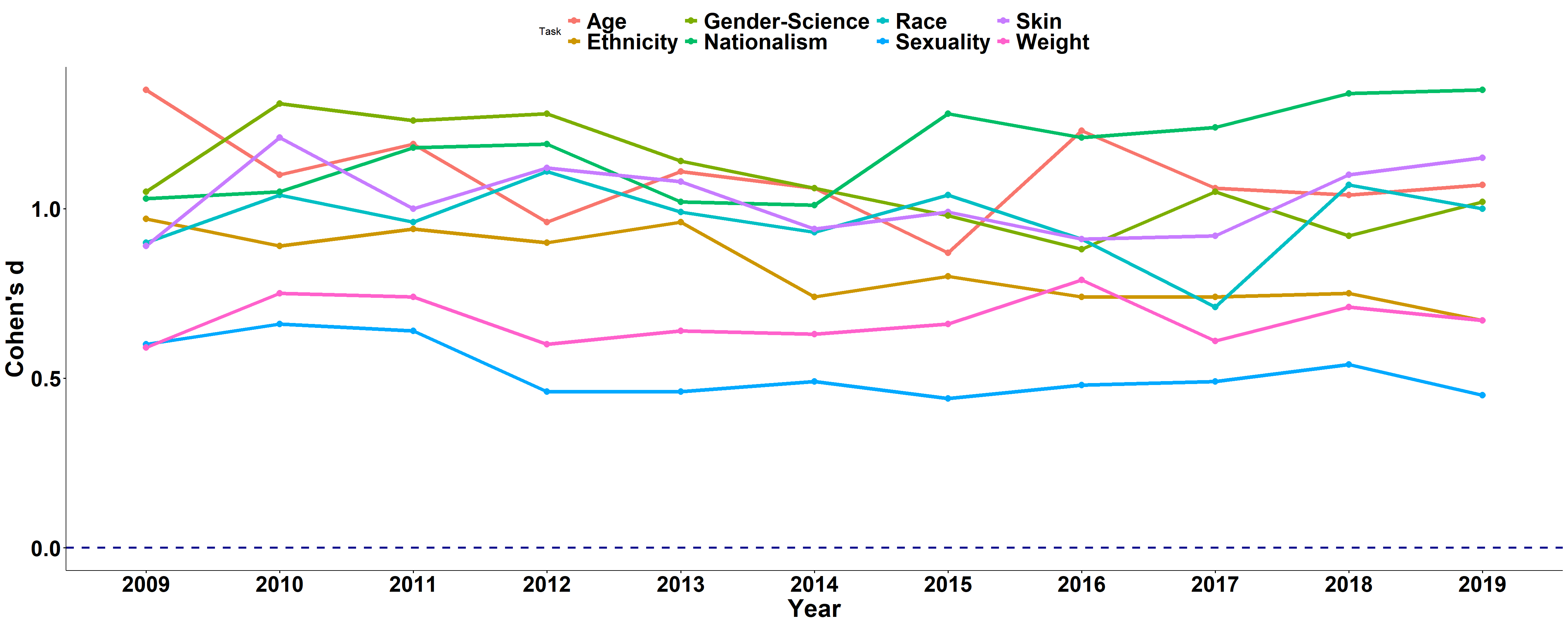
Self-Reported Direct Preference
att_df$Year = factor(att_df$Year, c("2009", "2010", "2011", "2012",
    "2013", "2014", "2015", "2016", "2017", "2018", "2019"))

pp <- ggline(att_df, x = "Year", y = "Cohens_d", ylab = "Cohen's d",
    color = "Task", size = 2)

pp <- pp + geom_hline(yintercept = 0, linetype = "dashed", color = "darkblue",
    size = 1.2)

pp <- pp + font("title", size = 20, color = "black", face = "bold") +
    font("legend.text", size = 25, color = "black", face = "bold") +
    font("xlab", size = 28, color = "black", face = "bold") +
    font("ylab", size = 28, color = "black", face = "bold") +
    font("xy.text", size = 25, color = "black", face = "bold")
# pp <- pp +theme(legend.position='none')

pp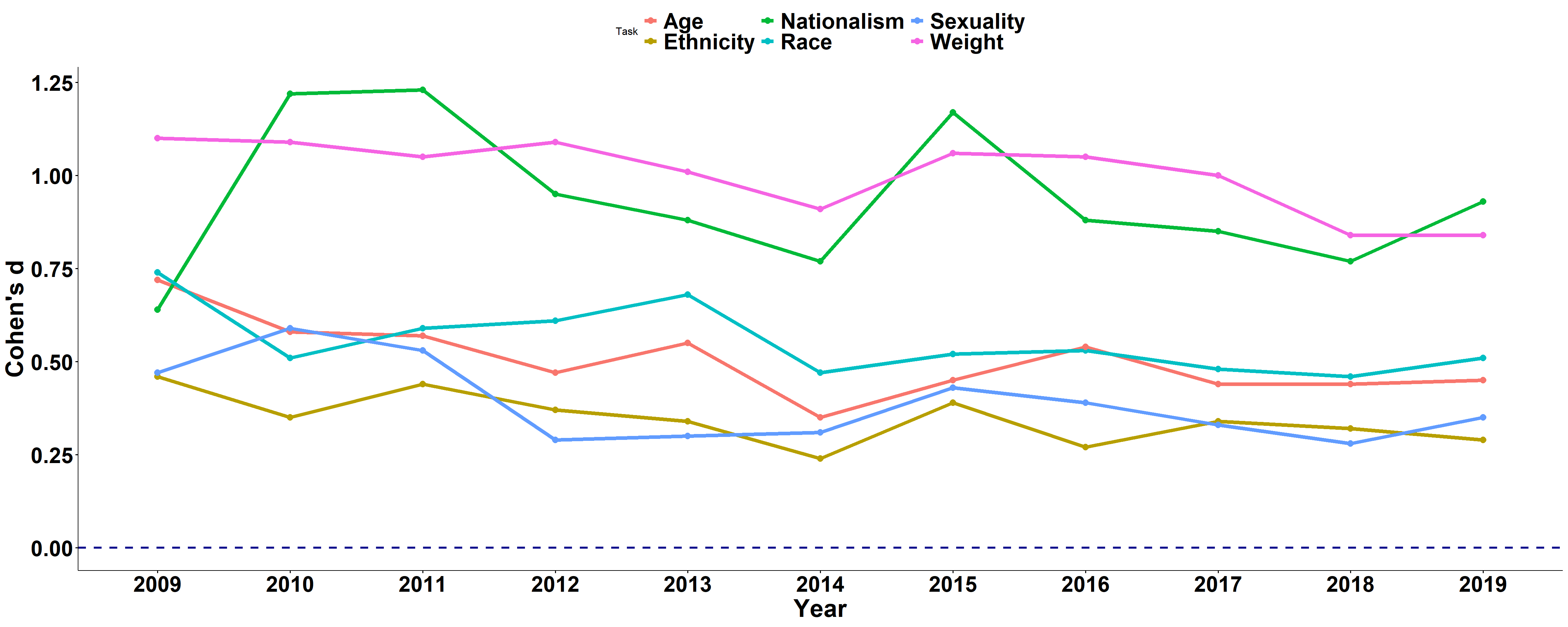
Self-Report: Feeling Thermometer Difference
thermo_df$Year = factor(thermo_df$Year, c("2009", "2010", "2011",
    "2012", "2013", "2014", "2015", "2016", "2017", "2018", "2019"))

pp <- ggline(thermo_df, x = "Year", y = "Cohens_d", ylab = "Cohen's d",
    color = "Task", size = 2)

pp <- pp + geom_hline(yintercept = 0, linetype = "dashed", color = "darkblue",
    size = 1.2)

pp <- pp + font("title", size = 20, color = "black", face = "bold") +
    font("legend.text", size = 25, color = "black", face = "bold") +
    font("xlab", size = 28, color = "black", face = "bold") +
    font("ylab", size = 28, color = "black", face = "bold") +
    font("xy.text", size = 25, color = "black", face = "bold")
# pp <- pp +theme(legend.position='none')

pp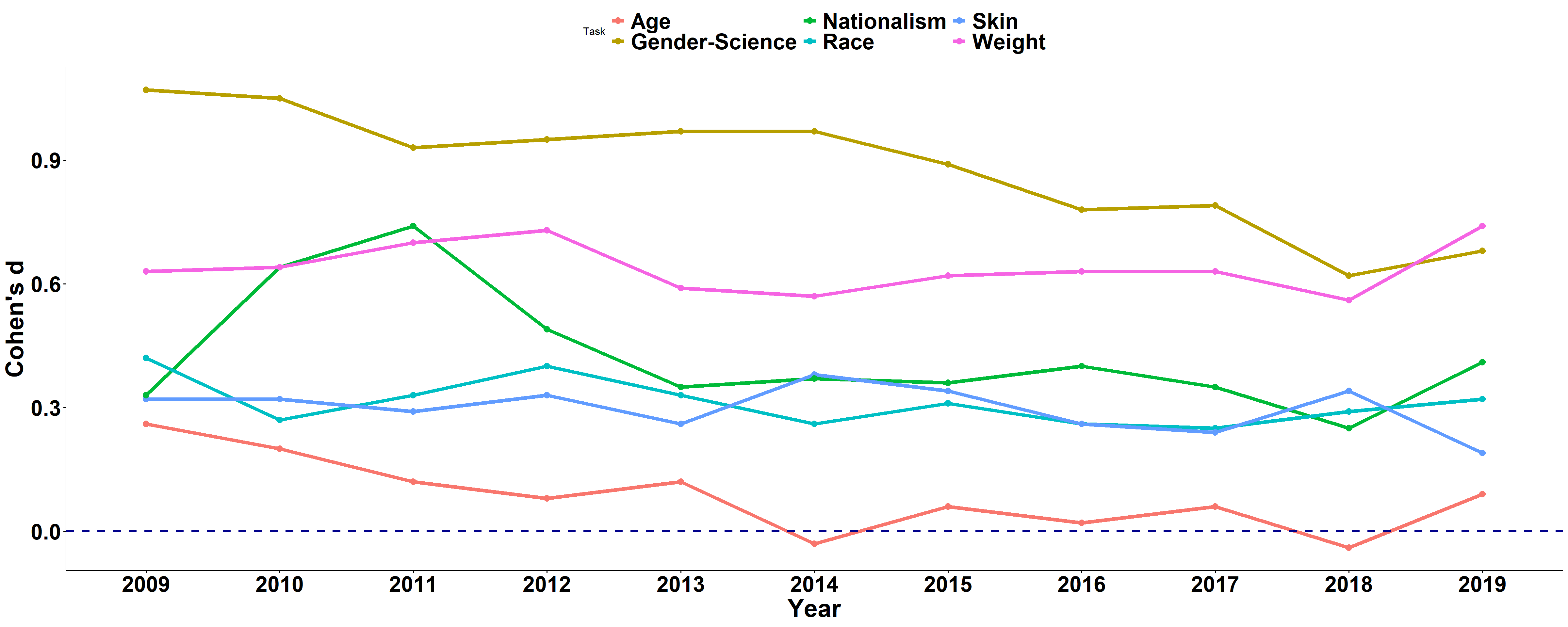
Summary
- Across all studies, Israelis were biased in their associations on both self-report and IAT, in favor of the dominant social groups.
- Across all tasks, the bias was much larger in the IAT than in self-report measures.
- The bias remained pretty much the same across the 12 years of data collection.
- IAT scores: The strongest bias among Israeli participants was in favor of Israel over the USA, and the smallest bias was for Straight people over Gay people.
Disclaimer
It is important to note that, currently, there is no consensus on the meaning of the IAT score. Some researchers would argue that it reflects an implicit or automatic bias in judgment, whereas others are more skeptical about this score and would say that automatic bias in judgment is only one factor that might influence the IAT score.
Show me more!
All the data, as well as the codebooks, are available on OSF.
Categories: Israel IAT Age-IAT Ethnicity-IAT Gender-Science IAT Nationalism-IAT Race-IAT Sexuality-IAT Skin-IAT Weight-IAT